Orthogonal frame via gram schmidt or eigendecomposition

Functions such as exp_x:T_xM→M require an orthonormal frame with respect to ℊ_x. We use the eigenvectors of ℊ_x find a set of orthonormal vectors. We begin with a numerical treatment. The scalar product considered has index 1.

MF[ℊ = Τ[Array[Random[] &, {3, 3}]] + Diag[{1, 1, -2}]]

( {{1.89258, 0.417475, 0.696925}, {0.417475, 1.33883, 0.530349}, {0.696925, 0.530349, -1.64054}} )

{d, V} = Eigensystem[ℊ]

{{2.30691, -1.8362, 1.12016}, {{-0.848536, -0.483587, -0.214781}, {-0.166597, -0.141103, 0.975877}, {0.502227, -0.863848, -0.0391664}}}

MF[α = T[Inv[Diag[Abs[d]^(1/2)] . V]]]

ListPlotVectorField3D[{{0, 0, 0}, #1} &/@α, ScaleFactor→.1, Frame→True, Axes→True] ;

( {{-0.55867, -0.31839, -0.14141}, {-0.122944, -0.10413, 0.72017}, {0.474526, -0.816202, -0.0370062}} )

[Graphics:../HTMLFiles/index_109.gif]

An orthonormal vector is in the column of α.

v = α[[1]]

ℊ . v . v

MF[Τα[ℊ, 0, T[α]]]

{-0.55867, -0.31839, -0.14141}

1.

( {{1., -1.38778*10^-16, -3.41741*10^-16}, {-1.38778*10^-16, -1., -1.45717*10^-16}, {-2.73219*10^-16, -4.85723*10^-17, 1.}} )

The above procedure is carried out by

MF[ΜOrthNormalize[ℊ]]

( {{-0.55867, -0.31839, -0.14141}, {-0.122944, -0.10413, 0.72017}, {0.474526, -0.816202, -0.0370062}} )

An alternative way to orthonormalize vectors is via gram schmidt. However, a basis of vectors of length ≠0 is required.

MF[Τα[ℊ, 0, T[ΜOrthNormalize[ℊ, Id[3]]]]]

( {{1., 0., 5.55112*10^-17}, {8.07018*10^-17, 1., 0.}, {4.03509*10^-17, -1.09665*10^-17, -1.}} )

Even in low dimensions, expressions get quite lengthy when solving the problem algebraically. As an example, a metric for a coordinate environment for the sphere.

assum = {0<x_1<ε, 0<x_2<ε, r>1} ;

f = {x_1, x_2, (r^2 - x_1^2 - x_2^2)^(1/2)}

df = Μd[f, 1, 2] ;

MF[ℊS2 = T[df] . df]

{x_1, x_2, (r^2 - x_1^2 - x_2^2)^(1/2)}

( {{1 + x_1^2/(r^2 - x_1^2 - x_2^2), (x_1 x_2)/(r^2 - x_1^2 - x_2^2)}, {(x_1 x_2)/(r^2 - x_1^2 - x_2^2), 1 + x_2^2/(r^2 - x_1^2 - x_2^2)}} )

ShowMat[{V = ΜOrthNormalize[ℊS2], Τα[ℊS2, 0, T[V]]}]

{( {{-x_2/(x_1^2 + x_2^2)^(1/2), x_1/(x_1^2 + x_2^2)^(1/2)}, {(x_1 (-1 + r^2/(x_1^2 + x_2^2))^(1/2))/r, (x_2 (-1 + r^2/(x_1^2 + x_2^2))^(1/2))/r}} ), ( {{1, 0}, {0, 1}} )}

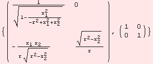
ShowMat[{V = ΜOrthNormalize[ℊS2, Id[2]], Τα[ℊS2, 0, T[V]]}]

{( {{1/(1 - x_1^2/(-r^2 + x_1^2 + x_2^2))^(1/2), 0}, {-(x_1 x_2)/(r (r^2 - x_2^2)^(1/2)), (r^2 - x_2^2)^(1/2)/r}} ), ( {{1, 0}, {0, 1}} )}

assum = {0<x_1<ε, 0<x_2<ε, r>1} ;

α = Inv[Diag[Abs[d]^(1/2)] . myV]//S

MF[Τα[ℊS2, 0, α]]//S

{{-x_2/(x_1^2 + x_2^2)^(1/2), (x_1 (-1 + r^2/(x_1^2 + x_2^2))^(1/2))/r}, {x_1/(x_1^2 + x_2^2)^(1/2), (x_2 (-1 + r^2/(x_1^2 + x_2^2))^(1/2))/r}}

( {{1, 0}, {0, 1}} )

Just for fun, we plot f(x_1,x_2) with emphasis on real and imaginary part.

τ = 1.2 ;

Plot3D[Evaluate[Re[f[[3]]/.r→1]], {x_1, -τ, τ}, {x_2, -τ, τ}, PlotPoints→40] ;

Plot3D[Evaluate[-Im[f[[3]]/.r→1]], {x_1, -τ, τ}, {x_2, -τ, τ}, PlotPoints→40] ;

[Graphics:../HTMLFiles/index_140.gif]

[Graphics:../HTMLFiles/index_141.gif]

The two parts attached are

Plot3D[Evaluate[Re[f[[3]]/.r→1] - Im[f[[3]]/.r→1]], {x_1, -τ, τ}, {x_2, -τ, τ}, PlotPoints→40] ;

Plot[Evaluate[Re[f[[3]]/.{x_2→0, r→1}] - Im[f[[3]]/.{x_2→0, r→1}]], {x_1, -τ, τ}] ;

[Graphics:../HTMLFiles/index_144.gif]

[Graphics:../HTMLFiles/index_145.gif]


Created by Mathematica  (December 22, 2006) Valid XHTML 1.1!